Predicting Fraudulent Claims from Accidents using Deep Learning - Part 1
Introduction
In today’s fast-paced world, insurance fraud has become a significant concern for insurance companies globally. Fraudulent claims not only lead to financial losses but also tarnish the reputation of insurers and increase premiums for honest policyholders. Among various types of insurance fraud, detecting fraudulent claims stemming from accidents poses a unique challenge due to the intricate nature of accidents and the diverse factors involved.
Traditional methods of fraud detection often rely on manual investigation and rule-based systems, which are time-consuming, labor-intensive, and may not be effective in uncovering sophisticated fraud schemes. However, with advancements in technology, particularly in the field of artificial intelligence and machine learning, insurers now have powerful tools at their disposal to combat insurance fraud more effectively. This blog post is divided into 2 parts, in Part 1, we experiment with different algorithms, and in Part 2 will develop and deploy a web-based App based on the results obtained in Part 1
Data loading
We begin by reading the insurance claims data as follows
# Load the data
data = pd.read_excel("claims.xlsx")
Data description
The insurance claim dataset contains information related to various insurance claims filed by policyholders. It includes details such as policyholder demographics, accident details, policy information, and claim outcomes. The dataset comprises the following columns:
Month: Month in which the claim was filed.
WeekOfMonth: Week number within the month when the claim was filed.
DayOfWeek: Day of the week when the claim was filed.
Make: Make of the vehicle involved in the accident.
AccidentArea: Area where the accident occurred.
DayOfWeekClaimed: Day of the week when the claim was reported.
MonthClaimed: Month when the claim was reported.
WeekOfMonthClaimed: Week number within the month when the claim was reported.
Sex: Gender of the policyholder.
MaritalStatus: Marital status of the policyholder.
Age: Age of the policyholder.
Fault: Fault attribution for the accident (e.g., policyholder, third party).
PolicyType: Type of insurance policy.
VehicleCategory: Category of the vehicle involved in the accident.
VehiclePrice: Price range of the vehicle.
FraudFound_P: Binary indicator for whether fraud was found in the claim.
PolicyNumber: Unique identifier for the insurance policy.
RepNumber: Representative number associated with the claim.
Deductible: Deductible amount for the claim.
DriverRating: Rating assigned to the driver involved in the accident.
Days_Policy_Accident: Number of days the policy has been active at the time of the accident.
Days_Policy_Claim: Number of days the policy has been active at the time of the claim.
PastNumberOfClaims: Number of claims filed in the past by the policyholder.
AgeOfVehicle: Age of the vehicle involved in the accident.
AgeOfPolicyHolder: Age of the policyholder.
PoliceReportFiled: Binary indicator for whether a police report was filed for the accident.
WitnessPresent: Binary indicator for whether a witness was present at the accident.
AgentType: Type of agent handling the claim.
NumberOfSuppliments: Number of supplementary items included in the claim.
AddressChange_Claim: Binary indicator for whether there was a change of address associated with the claim.
NumberOfCars: Number of cars involved in the accident.
Year: Year in which the claim was filed.
BasePolicy: Base policy associated with the claim.
ClaimSize: Size of the insurance claim.
Initial EDA
Let’s know our data by performing some explorations. We start by looking at the general overview of the data; the dimension of the data, the data types of the various columns, missing values, etc. This gives us an idea of what to expect and the necessary pre-processing, we can peek into the first few rows by doing this in Python
Data.head()
This operation gives us the first 10 rows of the data(Mostly there is little to see at this point). Next, the data.info() gives us an overview of the data as seen below
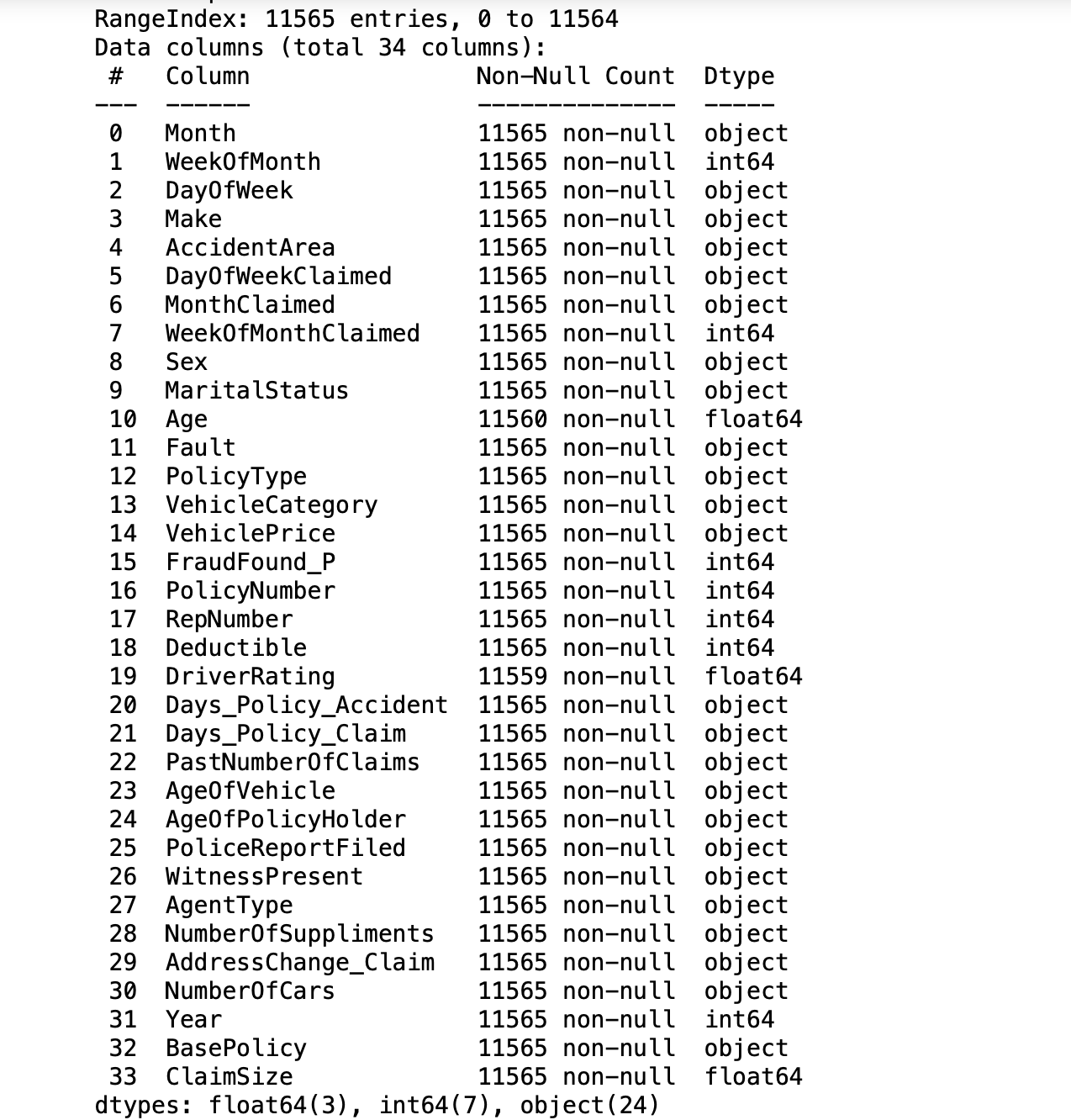
Looking at the result of the operation data.info, we can tell that there are 11565 data points with 34 columns. Out of these columns, 3 of them are of float type, 7 are integers and the rest 24 are objects. Furthermore, we can observe some missing values in some columns, specifically, there are missing values in Age and DriverRating. How many missing values are in these columns? we can find them out by this operation data.isnull().sum()
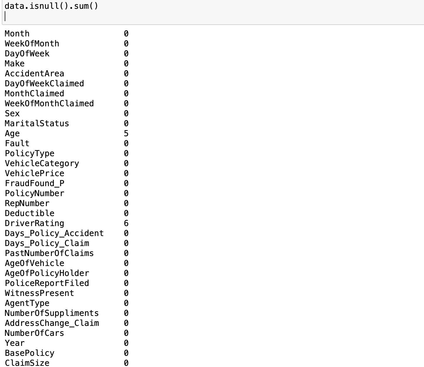 As we can see there are 5 missing values in Age and 6 missing values in DriverRating. It is a good thing that there are only a few missing values in the dataset). However, irrespective of this small number of missing values, we cannot proceed with our modeling without addressing this issue. We have to decide whether we are going to keep these data points or drop them(we will come back to this later). We examine the distribution of the target variable to understand the class balance in our task. Since our goal is to classify a claim as either legitimate or fraudulent, the target variable is FraudFound_P. FraudFound_P is a binary indicator for whether fraud was found in the claim or not (i.e 0 if there is no fraud and 1 if there is fraud). This
 (data['FraudFound_P'] == 1).sum() gives us the number of fraudulent claims whiles (data['FraudFound_P'] == 0).sum() gives us the number of legitimate claims. The results of the two operations show there are 10880 legitimate claims and only 685 fraudulent claims (not too surprising). In order words, only ~6\% of our datasets are fraudulent If you think about it, most of the claims filed will naturally be legitimate only a few will be fraudulent, same ideology can be extended to receiving spam emails. Most of your emails will be genuine and only a few will be in your spam folder. This phenomenon introduces us to what we call imbalanced data. Generally, if you have a split ratio of 90:10 in the variable of a binary classification, this is pretty obvious that the dataset is imbalanced
As you’ve already seen, a data imbalance is a classification problem where there is an unequal distribution of classes within the dataset.
As you will later see in this tutorial, we must handle the case of imbalances in the data. In the next section, we prepare our data for modeling including fixing the missing values, handling the class imbalance, converting column types into the appropriate types for the chosen algorithms etc
Data preparation and pre-processing
The first thing we want to address is that of the missing values. I have decided to keep these records, hence I need to choose an appropriate method to fill in these missing values (in the Age and DriverRating columns). I can impute these missing values using the mean, mode, or median values of the variable. I can also forward-fill or backward-fill with the last known or next value in that column.
This snippet data = data.fillna(method='ffill') shows that I’ve decided to forward-fill the missing values in my dataset.
Next, I want to change non-numerical datatypes to their numerical numerical representation. For instance, this data["Sex"] will give us a Male, Female, Female kinda response. What I want is to have them as binary responses 1 for male and 0 for female, you get the idea. The function below will help us achieve our desired results;
def convert_to_numerical(data):
    for col in data.select_dtypes(include=['object']).columns:
        unique_values = data[col].unique()
        value_map = {value: i+0 for i, value in enumerate(unique_values)}
        data[col] = data[col].map(value_map)
Calling the function convert_to_numerical on our data like this convert_to_numerical(data) will ensure that all non-numerical columns have been assigned their numerical representation. Doing this data["Sex"] will now give us 1,0,0 as desired.
On the issue of class imbalance, we can address it by either of the following; oversample the minority class, undersample the majority class, cost-sensitive learning, etc. Now will be a good time to handle the class imbalance, on second thought however, to understand the effect of the class imbalance in the dataset, we will continue to train and fit our model without addressing the imbalance constraint for now.
Model training
We start with a simple logistic model, where FraudFound_P is our target variable, and the rest of the columns as our predictor variables. Note that if we so desire, we can start with a simple confusion matrix to understand the relationship among the predictor variables and possible dimension reduction to include only needed features. However, this approach is not so necessary in our case as we will be employing deep learning for feature engineering, and we need to understand how each of the features will contribute to our final model We start with a simple logistic regression(with the class imbalance), as below;
#Logistic regression
from sklearn.model_selection import train_test_split
from sklearn.linear_model import LogisticRegression
from sklearn.metrics import confusion_matrix, accuracy_score

# Define features and target variable
X = data.drop(columns=['FraudFound_P'])
y = data['FraudFound_P']


# Split data into training and testing sets
X_train, X_test, y_train, y_test = train_test_split(X, y, test_size=0.2, random_state=42)

# Standardize features
scaler = StandardScaler()
X_train_scaled = scaler.fit_transform(X_train)
X_test_scaled = scaler.transform(X_test)

# Train logistic regression model with class weights
model = LogisticRegression()
model.fit(X_train_scaled, y_train)

# Make predictions on test data
y_pred = model.predict(X_test_scaled)

# Evaluate model performance
# Accuracy
accuracy = accuracy_score(y_test, y_pred)
print(accuracy)
The model has an accuracy of 94.07%. Not to be too happy, we inspect the class performance. We compute the confusion matrix to understand the performance of the model beyond the high accuracy
# Calculate confusion matrix
cm = confusion_matrix(y_test, y_pred)
class_names = ['Legit', 'Fraud']
# Plot confusion matrix
plt.figure(figsize=(8, 6))
sns.heatmap(cm, annot=True, cmap='Blues', fmt='g', cbar=False, annot_kws={"size": 14},
            xticklabels=['Predicted 0', 'Predicted 1'], yticklabels=['True 0', 'True 1'])
plt.xlabel('Predicted Label')
plt.ylabel('True Label')
plt.title('Confusion Matrix')
plt.xticks(ticks=np.arange(2) + 0.5, labels=class_names)
plt.yticks(ticks=np.arange(2) + 0.5, labels=class_names)
plt.show()
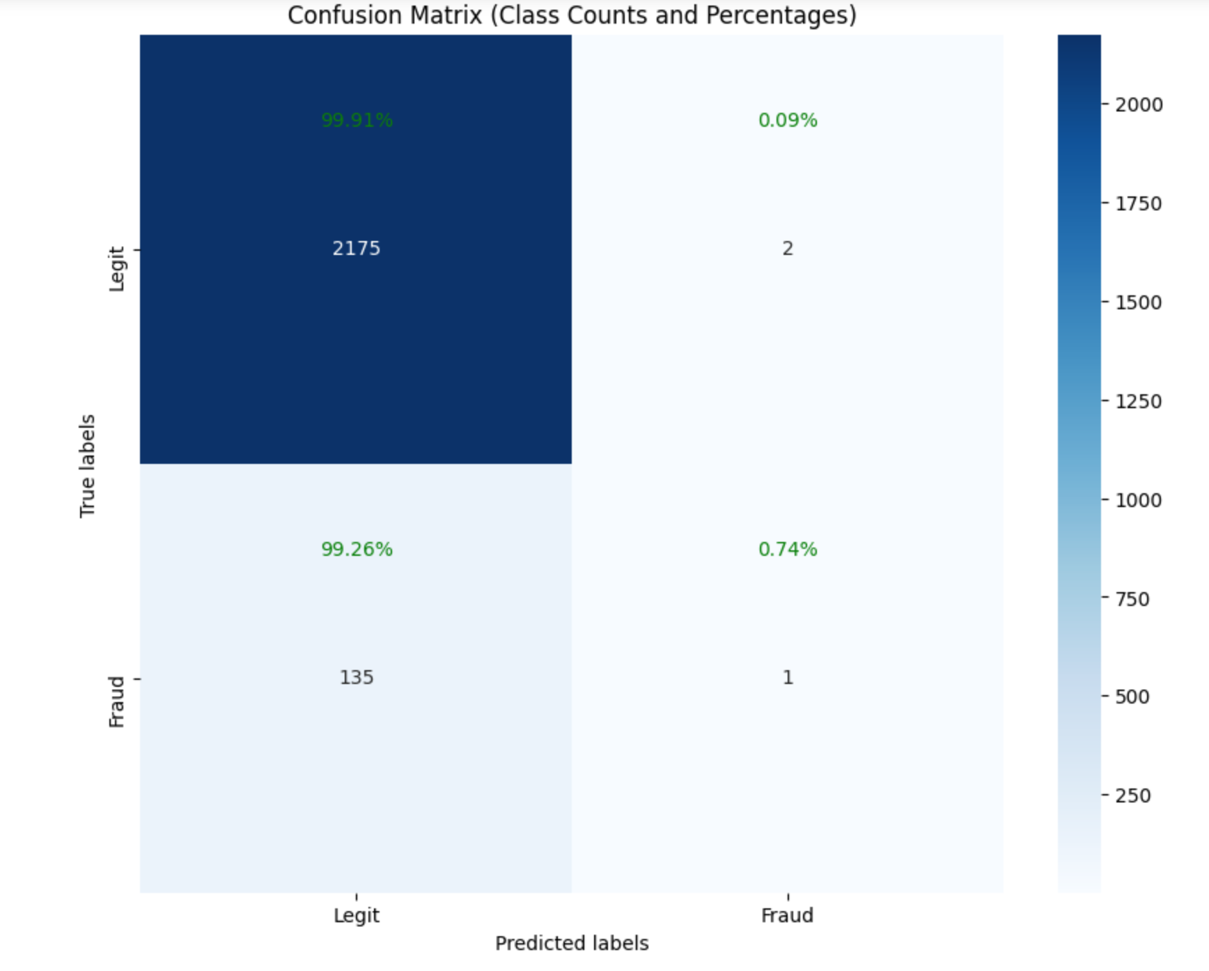 Observing the results of the confusion matrix from our model, it is clear that our model is doing well in predicting legitimate claims(99.9%) of the time. However this is not our task, our goal is to predict fraudulent claims which our model is so horrible at predicting (0.74%). The model is skewed toward the majority class, therefore despite the 94% accuracy recorded, our model has failed to solve the intended task. To address this is to address the imbalance problem in the dataset, to do this we will experiment with oversamplling the minority class, and adding class weights to the different classes accordingly.
We start with SMOTE which creates synthetic samples for the minority class. This way, we will increase the number of minority classes thereby solving the class imbalance issue
Observing the results of the confusion matrix from our model, it is clear that our model is doing well in predicting legitimate claims(99.9%) of the time. However this is not our task, our goal is to predict fraudulent claims which our model is so horrible at predicting (0.74%). The model is skewed toward the majority class, therefore despite the 94% accuracy recorded, our model has failed to solve the intended task. To address this is to address the imbalance problem in the dataset, to do this we will experiment with oversamplling the minority class, and adding class weights to the different classes accordingly.
We start with SMOTE which creates synthetic samples for the minority class. This way, we will increase the number of minority classes thereby solving the class imbalance issue
from imblearn.over_sampling import SMOTE
from sklearn.model_selection import train_test_split
from sklearn.linear_model import LogisticRegression
from sklearn.metrics import classification_report,accuracy_score,confusion_matrix
X_train, X_test, y_train, y_test = train_test_split(X, y, test_size=0.2, random_state=42)
smote = SMOTE(random_state=42)
X_train_resampled, y_train_resampled = smote.fit_resample(X_train, y_train)
model = LogisticRegression()
model.fit(X_train_resampled, y_train_resampled)
y_pred = model.predict(X_test)
print(classification_report(y_test, y_pred))
# Metrics
accuracy = accuracy_score(y_test, y_pred)
print(accuracy)
The model has an accuracy of 61%. As with the first model, we inspect the class performance with the confusion matrix to understand the performance of the model beyond the accuracy
# Calculate confusion matrix
cm = confusion_matrix(y_test, y_pred)
class_names = ['Legit', 'Fraud']
# Plot confusion matrix
plt.figure(figsize=(8, 6))
# Calculate class percentages
class_percentages = cm / cm.sum(axis=1)[:, np.newaxis]
# Plot confusion matrix with counts
sns.heatmap(cm, annot=True, fmt='d', cmap='Blues')
plt.xlabel('Predicted labels')
plt.ylabel('True labels')
plt.title('Confusion Matrix (Class Counts and Percentages)')
plt.xticks(ticks=np.arange(2) + 0.5, labels=class_names)
plt.yticks(ticks=np.arange(2) + 0.5, labels=class_names)

# Add text annotations for class percentages
for i in range(cm.shape[0]):
    for j in range(cm.shape[1]):
        # Compute percentage if count is not zero
        if cm[i, j] != 0:
            percentage = class_percentages[i, j]
            plt.text(j + 0.5, i + 0.2, f'{percentage:.2%}',
                     horizontalalignment='center', verticalalignment='center', color='green')

plt.show()
 The first thing we observe here is the drop in the overall accuracy from 94% to 61% just after solving the imbalance problem. Does this help solve our problem? Yes!, from not being able to predict any fraudulent claims in the previous model, we can predict 65 fraudulent claims as true fraudulent(True negatives). That notwithstanding, our model is still predicting some 71 fraudulent claims as legit (False negative). Our objective hereafter is to increase the number of fraudulent claims that are indeed predicted as fraudulent by reducing the number of false negative claims(reduce the 71 as low as possible) even if it means increasing the number of legit claims as fraudulent (False positive; 820 in our case). Think about it, it is better to predict legit claims as fraudulent which may turn out not to be fraudulent upon investigation rather than predicting a fraudulent claim as legit which could cause us to lose millions.
Now that we can deal with the class imbalance, we experiment with other models to reduce the false negatives.
Improving performance
We experiment with a different approach to handle class imbalance and observe the performance of the mode. We introduce the notion of class weights. In this approach, we assign weights to the Legit and Fraud classes; by assigning higher weights to the minority class(Fraud) and lower weights to the majority class(Legit), the model is trained to pay more attention to the minority class samples during the optimization process. In determining how to assign these weights, we use sklearn.utils to help compute them as below
from sklearn.utils.class_weight import compute_class_weight

# Calculate class weights
class_weights = compute_class_weight('balanced', classes=np.unique(y_train), y=y_train)

# Convert to dictionary format
class_weight = dict(zip(np.unique(y_train), class_weights))
print(class_weight)
Next, we add these class weights during the training of our model. To compare the performance, we add this class weights back to the logistic regression model as below and observe its performance thereafter.
#Logistic regression with weights

from sklearn.model_selection import train_test_split
from sklearn.linear_model import LogisticRegression
from sklearn.metrics import classification_report


# Train logistic regression model with class weights
model = LogisticRegression(class_weight=class_weight)
model.fit(X_train_scaled, y_train)

# Make predictions on test data
y_pred = model.predict(X_test_scaled)

# Evaluate model performance
print(classification_report(y_test, y_pred))
# Metrics
print(accuracy_score(y_test, y_pred))
When these blocks of code are executed, the first thing we notice about this approach to handling class imbalance is an improvement in the model performance from 61% to 67% overall accuracy. What about improvement in predicting fraudulent claims correctly? Well, that has improved significantly as well as observed from the confusion matrix below;
 In predicting fraudulent claims correctly, the new model has now predicted 105 claims correctly as fraudulent, which is an improvement over the previous 65 claims. This directly reduces the number of fraud claims misclassified as legit from 71 claims to 31 claims which is what we want. In general, there is an overall improvement in the performance of the class classification as observed from the previous confusion matrices.
However, 31 misclassified claims could still be high when we consider the monetary values (say a fraud classified as legit could result in thousands of dollars).
In the last sessions of this tutorial, we will take advantage of the time component of the dataset and experiment with a deep-learning sequential model to see if we can further reduce the number of false negatives and improve the general performance of the model. Additionally, we introduce different metrics such as recall, precision, and support which help us to determine how certain we are about our predictions
Hi. I am Bright Aboh; a data scientist, a climate change researcher and a music lover.