Predicting Fraudulent Accident Claims

data info

Introduction

In today’s fast-paced world, insurance fraud has become a significant concern for insurance companies globally. Fraudulent claims not only lead to financial losses but also tarnish the reputation of insurers and increase premiums for honest policyholders. Among various types of insurance fraud, detecting fraudulent claims stemming from accidents poses a unique challenge due to the intricate nature of accidents and the diverse factors involved.

Traditional methods of fraud detection often rely on manual investigation and rule-based systems, which are time-consuming, labor-intensive, and may not be effective in uncovering sophisticated fraud schemes. However, with advancements in technology, particularly in the field of artificial intelligence and machine learning, insurers now have powerful tools at their disposal to combat insurance fraud more effectively. This blog post is divided into 2 parts, in Part 1, we experiment with different algorithms, and in Part 2 will develop and deploy a web-based App based on the results obtained in Part 1

Data loading

We begin by reading the insurance claims data as follows

# Load the data
data = pd.read_excel("claims.xlsx")

Data description

The insurance claim dataset contains information related to various insurance claims filed by policyholders. It includes details such as policyholder demographics, accident details, policy information, and claim outcomes. The dataset comprises the following columns:

Month: Month in which the claim was filed.

WeekOfMonth: Week number within the month when the claim was filed.

DayOfWeek: Day of the week when the claim was filed.

Make: Make of the vehicle involved in the accident.

AccidentArea: Area where the accident occurred.

DayOfWeekClaimed: Day of the week when the claim was reported.

MonthClaimed: Month when the claim was reported.

WeekOfMonthClaimed: Week number within the month when the claim was reported.

Sex: Gender of the policyholder.

MaritalStatus: Marital status of the policyholder.

Age: Age of the policyholder.

Fault: Fault attribution for the accident (e.g., policyholder, third party).

PolicyType: Type of insurance policy.

VehicleCategory: Category of the vehicle involved in the accident.

VehiclePrice: Price range of the vehicle.

FraudFound_P: Binary indicator for whether fraud was found in the claim.

PolicyNumber: Unique identifier for the insurance policy.

RepNumber: Representative number associated with the claim.

Deductible: Deductible amount for the claim.

DriverRating: Rating assigned to the driver involved in the accident.

Days_Policy_Accident: Number of days the policy has been active at the time of the accident.

Days_Policy_Claim: Number of days the policy has been active at the time of the claim.

PastNumberOfClaims: Number of claims filed in the past by the policyholder.

AgeOfVehicle: Age of the vehicle involved in the accident.

AgeOfPolicyHolder: Age of the policyholder.

PoliceReportFiled: Binary indicator for whether a police report was filed for the accident.

WitnessPresent: Binary indicator for whether a witness was present at the accident.

AgentType: Type of agent handling the claim.

NumberOfSuppliments: Number of supplementary items included in the claim.

AddressChange_Claim: Binary indicator for whether there was a change of address associated with the claim.

NumberOfCars: Number of cars involved in the accident.

Year: Year in which the claim was filed.

BasePolicy: Base policy associated with the claim.

ClaimSize: Size of the insurance claim.

Data intro

Let’s know our data by performing some explorations. We start by looking at the general overview of the data; the dimension of the data, the data types of the various columns, missing values, etc. This gives us an idea of what to expect and the necessary pre-processing, we can peek into the first few rows by doing this in Python

Data.head()

This operation gives us the first 10 rows of the data(Mostly there is little to see at this point). Next, the data.info() gives us an overview of the data as seen below data info

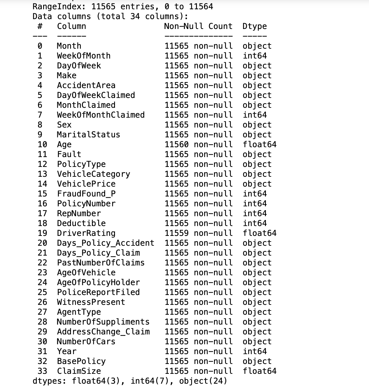
Looking at the result of the operation data.info, we can tell that there are 11565 data points with 34 columns. Out of these columns, 3 of them are of float type, 7 are integers and the rest 24 are objects. Furthermore, we can observe some missing values in some columns, specifically, there are missing values in Age and DriverRating. How many missing values are in these columns? we can find them out by this operation data.isnull().sum()

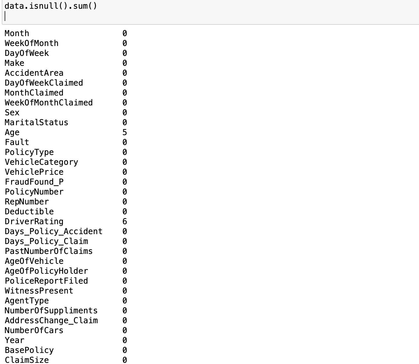data info As we can see there are 5 missing values in Age and 6 missing values in DriverRating. It is a good thing that there are only a few missing values in the dataset). However, irrespective of this small number of missing values, we cannot proceed with our modeling without addressing this issue. We have to decide whether we are going to keep these data points or drop them(we will come back to this later). We examine the distribution of the target variable to understand the class balance in our task. Since our goal is to classify a claim as either legitimate or fraudulent, the target variable is FraudFound_P. FraudFound_P is a binary indicator for whether fraud was found in the claim or not (i.e 0 if there is no fraud and 1 if there is fraud). This (data['FraudFound_P'] == 1).sum() gives us the number of fraudulent claims whiles (data['FraudFound_P'] == 0).sum() gives us the number of legitimate claims. The results of the two operations show there are 10880 legitimate claims and only 685 fraudulent claims (not too surprising). In order words, only ~6\% of our datasets are fraudulent If you think about it, most of the claims filed will naturally be legitimate only a few will be fraudulent, same ideology can be extended to receiving spam emails. Most of your emails will be genuine and only a few will be in your spam folder. This phenomenon introduces us to what we call imbalanced data. Generally, if you have a split ratio of 90:10 in the variable of a binary classification, this is pretty obvious that the dataset is imbalanced

As you’ve already seen, a data imbalance is a classification problem where there is an unequal distribution of classes within the dataset.

As you will later see in this tutorial, we must handle the case of imbalances in the data. In the next section, we prepare our data for modeling including fixing the missing values, handling the class imbalance, converting column types into the appropriate types for the chosen algorithms etc

Data preparation and pre-processing

The first thing we want to address is that of the missing values. I have decided to keep these records, hence I need to choose an appropriate method to fill in these missing values (in the Age and DriverRating columns). I can impute these missing values using the mean, mode, or median values of the variable. I can also forward-fill or backward-fill with the last known or next value in that column. Additionally, the functions below also process the object type data(e.g assigning numerical values to months of the year) by assigning numerical values to the non-numerical and categorical data.

#Preprocessing functions
import pandas as pd

# Load your dataset
def load_data(file_path):
    data = pd.read_excel(file_path)
    return data.copy()

# Function to process month columns
def process_months(df, month_columns):
    months = {
        'Jan': 1, 'Feb': 2, 'Mar': 3, 'Apr': 4, 'May': 5, 'Jun': 6,
        'Jul': 7, 'Aug': 8, 'Sep': 9, 'Oct': 10, 'Nov': 11, 'Dec': 12
    }
    month_proc = lambda x: months.get(x, 0)
    
    for col in month_columns:
        df[col] = df[col].apply(month_proc)
    return df

# Function to process day of week columns
def process_days_of_week(df, day_columns):
    days = {
        'Monday': 1, 'Tuesday': 2, 'Wednesday': 3,
        'Thursday': 4, 'Friday': 5, 'Saturday': 6, 'Sunday': 7
    }
    day_proc = lambda x: days.get(x, 0)
    
    for col in day_columns:
        df[col] = df[col].apply(day_proc)
    return df

# Function to process vehicle price
def process_vehicle_price(df, vehicle_price_column):
    vehicle_prices = {
        'less than 20000': 1, '20000 to 29000': 2, '30000 to 39000': 3,
        '40000 to 59000': 4, '60000 to 69000': 5, 'more than 69000': 6,
    }
    vehicle_price_proc = lambda x: vehicle_prices.get(x, 0)
    
    df[vehicle_price_column] = df[vehicle_price_column].apply(vehicle_price_proc)
    return df

# Function to process vehicle age
def process_vehicle_age(df, vehicle_age_column):
    AgeOfVehicle_variants = {
        'new': 0.5, '2 years': 2, '3 years': 3, '4 years': 4,
        '5 years': 5, '6 years': 6, '7 years': 7, 'more than 7': 8.5,
    }
    vehicle_age_proc = lambda x: AgeOfVehicle_variants[x]
    
    df[vehicle_age_column] = df[vehicle_age_column].apply(vehicle_age_proc)
    return df

# Function to process policy holder age
def process_policy_holder_age(df, age_column):
    age_variants = {
        '16 to 17': 1, '18 to 20': 2, '21 to 25': 3, '26 to 30': 4,
        '31 to 35': 5, '36 to 40': 6, '41 to 50': 7, '51 to 65': 8, 'over 65': 9,
    }
    age_proc = lambda x: age_variants[x]
    
    df[age_column] = df[age_column].apply(age_proc)
    return df

# Function to fill missing values
def fill_missing_values(df, columns_with_default_values):
    for column, default_value in columns_with_default_values.items():
        df[column] = df[column].fillna(default_value)
    return df

# Main processing function
def process_data(file_path):
    df = load_data(file_path)
    
    df = process_months(df, ['Month', 'MonthClaimed'])
    df = process_days_of_week(df, ['DayOfWeek', 'DayOfWeekClaimed'])
    df = process_vehicle_price(df, 'VehiclePrice')
    df = process_vehicle_age(df, 'AgeOfVehicle')
    df = process_policy_holder_age(df, 'AgeOfPolicyHolder')
    
    df = fill_missing_values(df, {'Age': df['Age'].mean(), 'DriverRating': df['DriverRating'].mean()})
    
    return df

# File path to the dataset
file_path = "claims.xlsx"

# Process the data
df_processed = process_data(file_path)

Calling the main processing function convert_to_numerical on our data like this convert_to_numerical(data) will ensure that all non-numerical columns have been assigned their numerical representation. Doing this data["Sex"] will now give us 1,0,0 as desired.

Initial Data Exploratory Analysis(DEA)

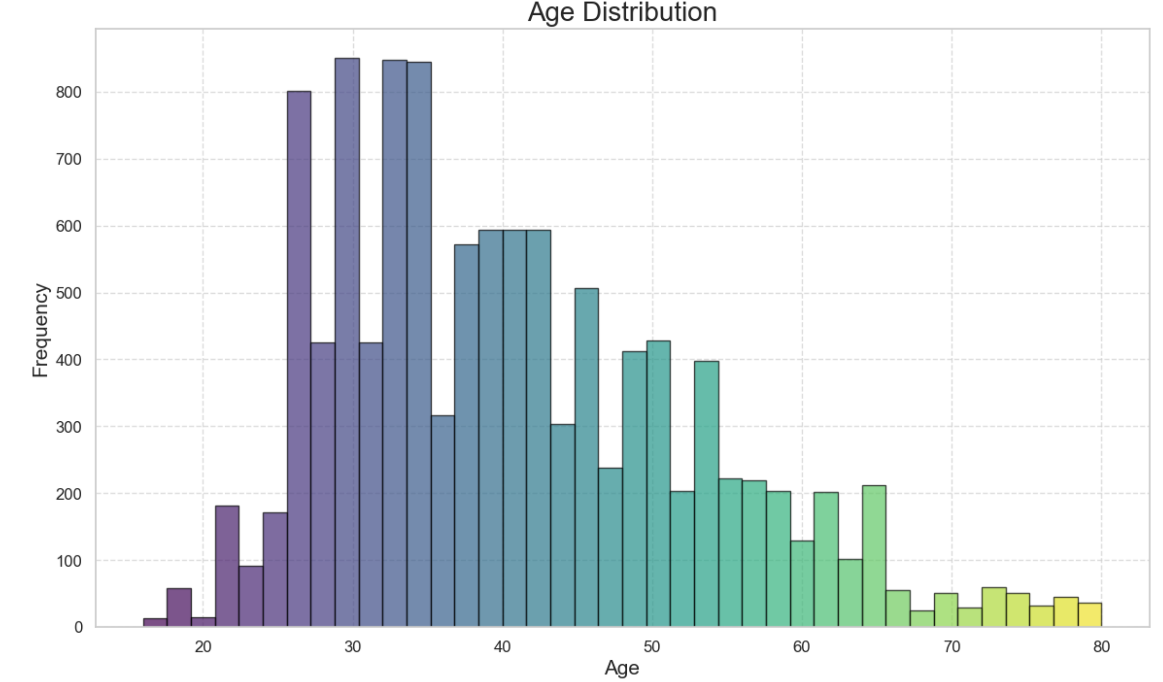
Next, we look at how the distribution of some of the columns and their relationship with the target variable(FraudFound_P). First of all, we look at the age distribution within the dataset with the following snippet;

import pandas as pd
import numpy as np
import matplotlib.pyplot as plt
import seaborn as sns

# Sample data

# Set the style
sns.set(style="whitegrid")

# Create figure and axis
plt.figure(figsize=(14, 8))

# Plot histogram
n, bins, patches = plt.hist(df_processed['Age'], bins=40, edgecolor='black', alpha=0.7)

# Add colors
for i in range(len(patches)):
    patches[i].set_facecolor(plt.cm.viridis(i / len(patches)))

# Add title and labels
plt.title('Age Distribution', fontsize=20)
plt.xlabel('Age', fontsize=15)
plt.ylabel('Frequency', fontsize=15)

# Add grid
plt.grid(True, linestyle='--', alpha=0.7)

# Customize ticks
plt.xticks(fontsize=12)
plt.yticks(fontsize=12)

# Show the plot
plt.show()

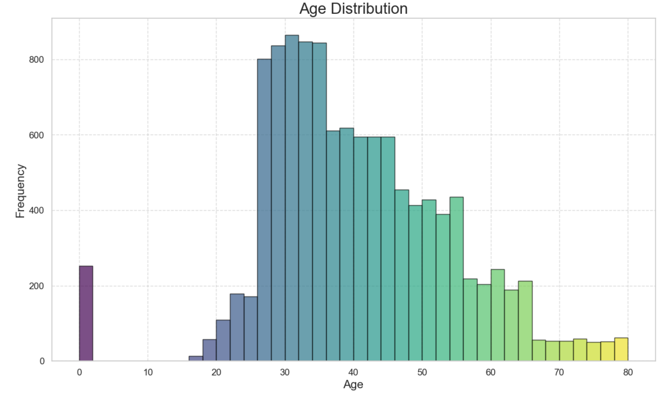data info From the graph above, see close to 300 claims with 0 years which doesn’t make sense, as babies don’t drive. We replace these records with the mean age within the dataset by the following snippet of code;

##Drop age 0 as babies dont drive
# Calculate the median age of the drivers
median_age = df_processed[df_processed['Age'] != 0]['Age'].median()

# Replace the age values that are 0 with the median age
df_processed['Age'] = df_processed['Age'].replace(0, median_age)

data info The result shows 0 years replaced with the mean of the ages.

Secondly, we can have an insight into the age distribution with fraudulent claims. The snippet code below shows which ages are more likely to have a fraudulent claim. To achieve this, we plot the Kernel Density Estimation graph as follows;

# Set the style
sns.set(style="whitegrid")

# Create FacetGrid
g = sns.FacetGrid(df_processed, hue='FraudFound_P', height=7, aspect=2, palette='viridis')

# Map the KDE plot to the grid
g.map(sns.kdeplot, 'Age', shade=True)

# Add a title
plt.title('Age Distribution for Fraud and No Fraud Claims', fontsize=20)

# Add legend
g.add_legend(title="Fraud Found")

# Customize ticks and labels
plt.xlabel('Age', fontsize=15)
plt.ylabel('Density', fontsize=15)
plt.xticks(fontsize=12)
plt.yticks(fontsize=12)


ax = plt.gca()
for i, line in enumerate(ax.get_lines()):
    x_data = line_get_xdata()
    y_data = line_get_ydata()
    peak_index = np.argmax(ydata)
    peak_x = x_data[peak_index]
    peak_y = y_data[peak_index]
    ax.fill_between(x_data, 0, y_data, where = (x_data<=peak_x), colors = 'red', alpha = 0.3)
    

# Show the plot
plt.show()

data info

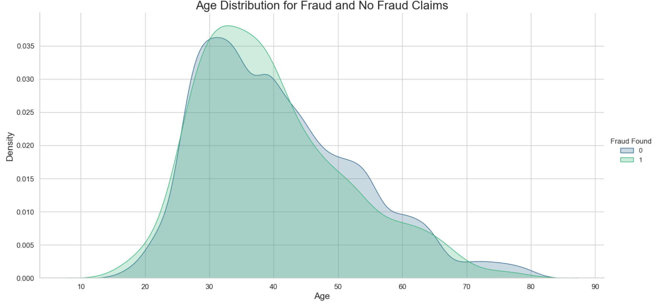
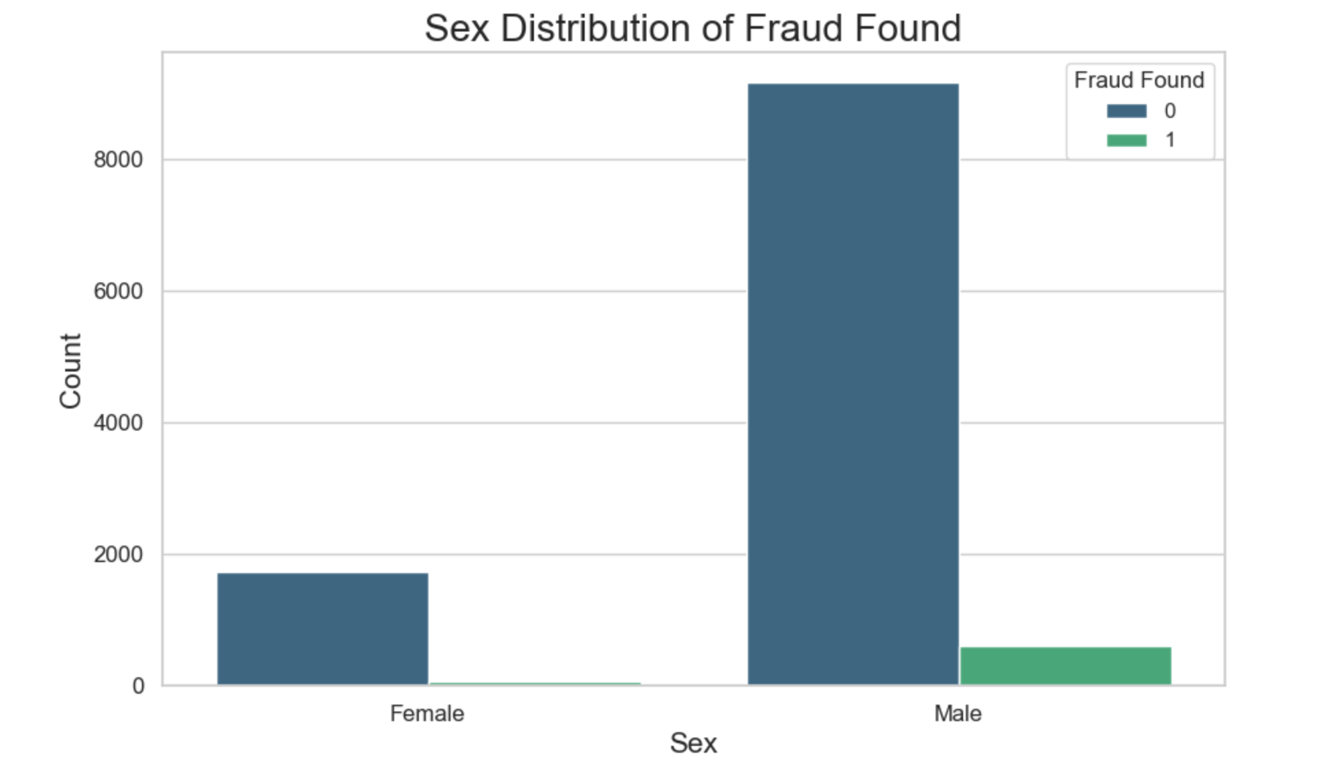
The results show that most of the fraudulent claims are around the 30-40 year brackets. This makes sense since the age of most of the drivers in this dataset are in this age group. Another interesting insight we could drive is to investigate the distribution of fraudulent claims across the sex of the drivers.

import seaborn as sns
import matplotlib.pyplot as plt

# Assuming 'data' is your DataFrame and 'Sex' and 'FraudFound_P' are columns in it
plt.figure(figsize=(10, 6))
sns.countplot(x='Sex', hue='FraudFound_P', data=df_processed, palette='viridis')

# Add title and labels
plt.title('Sex Distribution of Fraud Found', fontsize=20)
plt.xlabel('Sex', fontsize=15)
plt.ylabel('Count', fontsize=15)

# Customize ticks and labels
plt.xticks(fontsize=12)
plt.yticks(fontsize=12)

# Add legend
plt.legend(title='Fraud Found')

# Show the plot
plt.show()

What we observe is that there are a lot more fraudulent claimers who are males. Without looking at the sex distribution within the dataset as a whole, one may be tempted to say that male drivers are more likely to commit fraudulent claims than their female counterparts. If we look at the sex distribution, we see that male drivers outnumber female drivers hence the possibility to find more fraudulent claims in the male category. data info

What about the car makes that are frequently involved in fraudulent claims? Can that be established? The snippet of code below provides an insight of the car makes which are frequently involved in fraudulent claims.

import seaborn as sns
import matplotlib.pyplot as plt
import pandas as pd

fraud_rate_make = df_processed.groupby('Make').agg({
    "FraudFound_P": "mean", 
    "PolicyNumber": 'count'
})
fraud_rate_make.columns = ['FraudRate', 'Count']
fraud_rate_make = fraud_rate_make.apply(lambda x: round(x, 3))
fraud_rate_make = fraud_rate_make.sort_values(by='FraudRate', ascending=False)

# Reset index to turn 'Make' into a column for easier plotting
fraud_rate_make.reset_index(inplace=True)

# Plotting
plt.figure(figsize=(12, 8))
barplot = sns.barplot(x='FraudRate', y='Make', data=fraud_rate_make, palette='viridis')

# Add counts to the bars
for index, value in enumerate(fraud_rate_make['FraudRate']):
    barplot.text(value, index, f'{value:.2%}', color='black', ha="left", va="center")

# Add title and labels
plt.title('Fraud Rate by Make', fontsize=20)
plt.xlabel('Fraud Rate', fontsize=15)
plt.ylabel('Make', fontsize=15)

# Show the plot
plt.show()

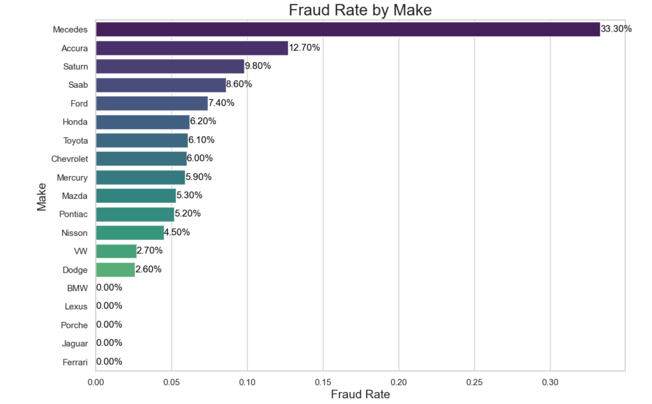data info The analysis reveals that Mercedes cars accounted for 33.30% of all fraudulent claims detected, making it the most implicated car make. Accura followed with 12.70% of fraudulent claims. This data underscores the importance of monitoring and investigating claims associated with these car makes to combat insurance fraud effectively.

Another aspect to consider is analyzing the WitnessPresent column to gain insights into how the presence of a witness contributes to fraud cases. To achieve this; we use this block of codes

import pandas as pd
import matplotlib.pyplot as plt



# Filter data where FraudFound_P is 1
df_fraud = df_processed[df_processed['FraudFound_P'] == 1]

# Group data by 'WitnessPresent' and count the number of policies
count_rep_wit = df_fraud.groupby('WitnessPresent').agg({
    "PolicyNumber": 'count'
}).reset_index()

# Rename columns
count_rep_wit.columns = ['WitnessPresent', 'Count']

# Plot the bar graph
plt.figure(figsize=(10, 6))
sns.barplot(x='WitnessPresent', y='Count', data=count_rep_wit, palette='viridis')

# Add labels to each bar
for index, row in count_rep_wit.iterrows():
    plt.text(row.name, row['Count'], row['Count'], color='black', ha="center", va="bottom")

# Add title and labels
plt.title('Count of Policies by Witness Presence in Fraud Cases', fontsize=20)
plt.xlabel('Witness Present', fontsize=15)
plt.ylabel('Count of Policies', fontsize=15)

# Customize ticks and labels
plt.xticks(ticks=[0, 1], labels=['No', 'Yes'], fontsize=12)
plt.yticks(fontsize=12)

# Show the plot
plt.show()

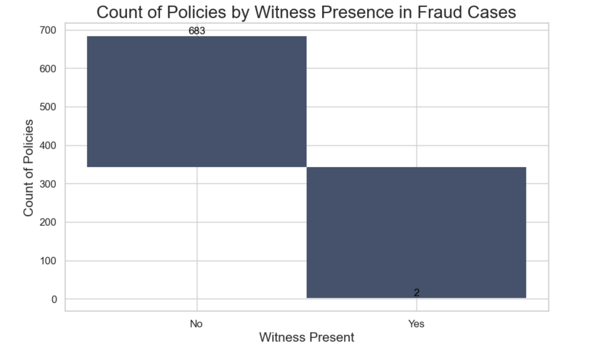data info We observe an interesting trend: out of 685 fraudulent claims, 683 (representing 99.7%) occurred at locations where no witnesses were present, and only 2 fraudulent claims had witnesses present. This suggests that, in the absence of witnesses at the accident scene, a claim is highly likely to be fraudulent.

Next, we examine the distribution of claim sizes in relation to fraudulent cases. Can we discern any patterns from this analysis? To explore this question, we’ll utilize the following snippet.

# Replace negative claim sizes and zeros with NaN
df_processed['ClaimSize'] = df_processed['ClaimSize'].apply(lambda x: np.nan if x <= 0 else x)

# Calculate the mean claim size excluding NaN values
mean_claim_size = df_processed['ClaimSize'].mean()

# Replace NaN values with the mean claim size
df_processed['ClaimSize'].fillna(mean_claim_size, inplace=True)


# Create FacetGrid for visualization
g = sns.FacetGrid(df_processed, hue='FraudFound_P', height=7, aspect=2, palette='viridis')

# Map the KDE plot to the grid
g.map(sns.kdeplot, 'ClaimSize', shade=True)

# Add title
plt.title('ClaimSize Distribution for Fraud and No Fraud Claims', fontsize=20)

# Add legend
g.add_legend(title='Fraud Found')

# Customize ticks and labels
plt.xlabel('Claim Size', fontsize=15)
plt.ylabel('Density', fontsize=15)
plt.xticks(fontsize=12)
plt.yticks(fontsize=12)

# Add vertical line for minimum claim size
min_claim_size = df_processed['ClaimSize'].min()
plt.axvline(x=min_claim_size, color='red', linestyle='--', label=f'Min Claim Size: {min_claim_size}')
plt.legend()

# Show the plot
plt.show()

data info

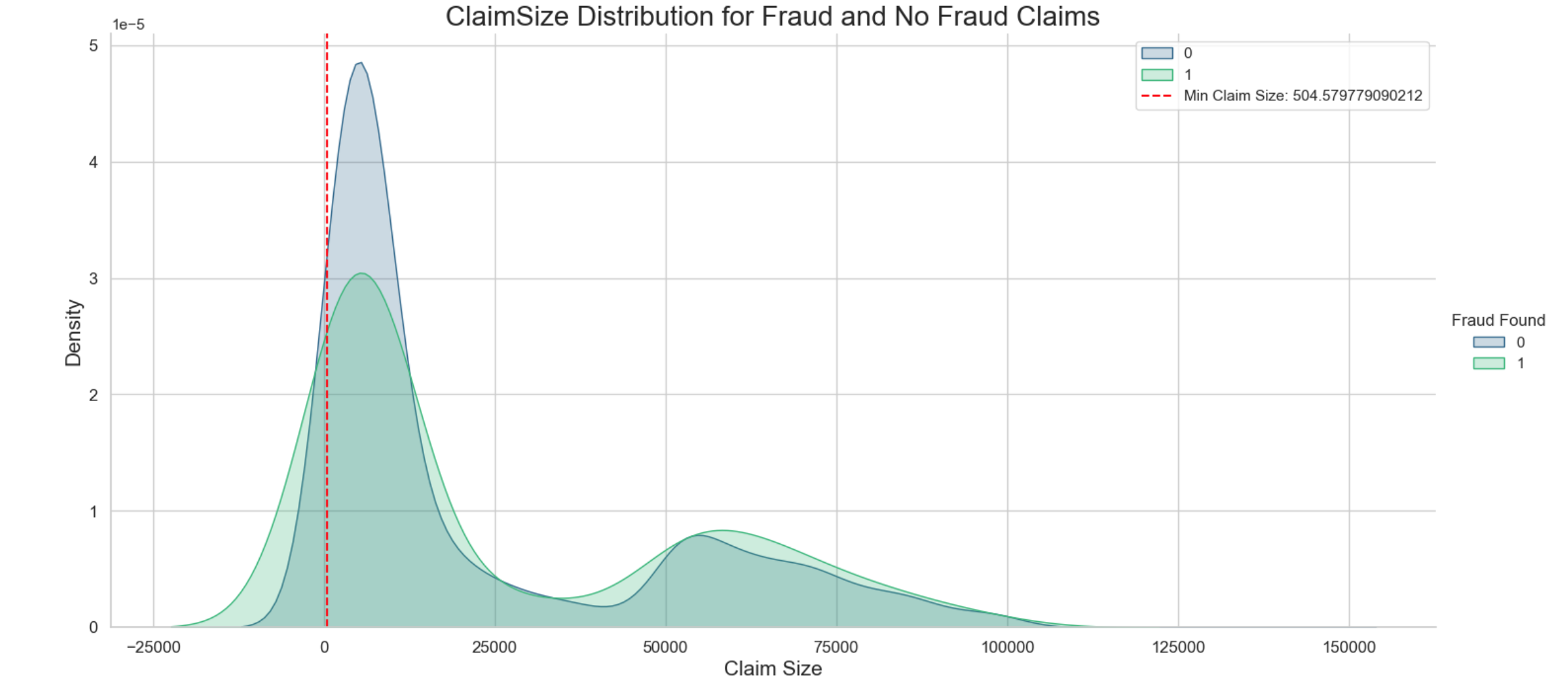
The findings reveal that legitimate claims surpass fraudulent ones in terms of dollar values and counts. This suggests a notable disparity in financial magnitude between the two types of claims. Lower fraud claim sizes may also indicate that these claims could potentially go unnoticed.

Machine learning

We are embarking on a critical investigation into whether we can develop a robust machine learning model using various dataset features to predict potential fraudulent insurance claims. By integrating pertinent attributes, our goal is to construct a predictive framework that can identify patterns indicative of fraudulent activities. This exploration not only aims to bolster fraud detection capabilities but also underscores the efficacy of advanced analytical techniques in combating deceptive claims within the insurance sector. To achieve this, we will employ logistic regression, XGBoost, and random forest classifiers.

Our methodology involves a systematic approach where each dataset feature is sequentially added to the model. If a feature does not improve the model’s performance, it is removed. Conversely, features that enhance overall model performance are retained. This iterative process continues until all 34 features have been evaluated, ensuring that only the most impactful features are selected for final model predictions.

Logistic model

We start with a simple logistic model, where FraudFound_P is our target variable, and the rest of the columns as our predictor variables.

import pandas as pd
import numpy as np
import matplotlib.pyplot as plt
import seaborn as sns
from sklearn.pipeline import Pipeline
from sklearn.compose import ColumnTransformer
from sklearn.impute import SimpleImputer
from sklearn.preprocessing import StandardScaler
from sklearn.metrics import classification_report, roc_curve, auc, confusion_matrix
from sklearn.model_selection import train_test_split, cross_val_predict, GridSearchCV
from sklearn.linear_model import LogisticRegression
from sklearn.utils.class_weight import compute_class_weight


# Assign unique integer values to all non-numeric values in the DataFrame
for col in df_processed.select_dtypes(include=['object']).columns:
    unique_values = df_processed[col].unique()
    value_map = {value: i for i, value in enumerate(unique_values)}
    df_processed[col] = df_processed[col].map(value_map)

# Define features and target
X = df_processed.drop('FraudFound_P', axis=1)
y = df_processed['FraudFound_P']

# Split the data into training and testing sets with stratify
X_train, X_test, y_train, y_test = train_test_split(X, y, test_size=0.3, random_state=42, stratify=y)

# Compute class weights based on the training set
class_weights = compute_class_weight(class_weight='balanced', classes=np.unique(y_train), y=y_train)
class_weights_dict = {i: class_weights[i] for i in range(len(class_weights))}
print(class_weights_dict)

# Initialize variables for the stepwise feature selection
best_features = []
best_score = 0
threshold_score = 0.5

# Define the logistic regression parameters for Grid Search
param_grid = {
    'classifier__C': [0.01, 0.1, 1, 10],
    'classifier__solver': ['liblinear', 'lbfgs']
}

# Iterate over all features
for feature in X.columns:
    # Add the new feature to the list of best features
    features_to_try = best_features + [feature]
    
    # Create a pipeline with the current set of features
    current_pipeline = Pipeline(steps=[
        ('preprocessor', ColumnTransformer(
            transformers=[
                ('num', Pipeline(steps=[
                    ('imputer', SimpleImputer(strategy='median')),
                    ('scaler', StandardScaler())
                ]), X[features_to_try].select_dtypes(include=['float64', 'int64']).columns),
                ('cat', Pipeline(steps=[
                    ('imputer', SimpleImputer(strategy='constant', fill_value=0))
                ]), X[features_to_try].select_dtypes(include=['int']).columns)
            ]
        )),
        ('classifier', LogisticRegression(random_state=42, max_iter=10000, class_weight=class_weights_dict))
    ])
    
    # Setup Grid Search with cross-validation
    grid_search = GridSearchCV(current_pipeline, param_grid, cv=5, scoring='roc_auc', n_jobs=-1, verbose=0)
    
    # Fit the model
    grid_search.fit(X_train[features_to_try], y_train)
    
    # Get the best score
    score = grid_search.best_score_
    
    # If the performance improves and is above the threshold, keep the feature
    if score > best_score and score >= threshold_score:
        best_score = score
        best_features.append(feature)
        print(f"Added feature: {feature} - New best score: {best_score}")

# Print the final set of best features
print("Best set of features: ", best_features)

# Create a final pipeline with the best features
final_pipeline = Pipeline(steps=[
    ('preprocessor', ColumnTransformer(
        transformers=[
            ('num', Pipeline(steps=[
                ('imputer', SimpleImputer(strategy='median')),
                ('scaler', StandardScaler())
            ]), X[best_features].select_dtypes(include=['float64', 'int64']).columns),
            ('cat', Pipeline(steps=[
                ('imputer', SimpleImputer(strategy='constant', fill_value=0))
            ]), X[best_features].select_dtypes(include=['int']).columns)
        ]
    )),
    ('classifier', LogisticRegression(random_state=42, max_iter=10000, class_weight=class_weights_dict))
])

# Fit the final pipeline with the best features
final_pipeline.fit(X_train[best_features], y_train)

# Predict and evaluate using the final model
y_pred = final_pipeline.predict(X_test[best_features])
print(classification_report(y_test, y_pred))

# Generate cross-validated predictions for ROC AUC curve using the best model
y_scores = cross_val_predict(final_pipeline, X[best_features], y, cv=5, method='predict_proba')[:, 1]

# Compute ROC curve and ROC AUC
fpr, tpr, thresholds = roc_curve(y, y_scores)
roc_auc = auc(fpr, tpr)

# Plot ROC AUC curve
plt.figure(figsize=(8, 6))
plt.plot(fpr, tpr, color='darkorange', lw=2, label='ROC curve (area = %0.2f)' % roc_auc)
plt.plot([0, 1], [0, 1], color='navy', lw=2, linestyle='--')
plt.xlim([0.0, 1.0])
plt.ylim([0.0, 1.05])
plt.xlabel('False Positive Rate')
plt.ylabel('True Positive Rate')
plt.title('Receiver Operating Characteristic (ROC) Curve')
plt.legend(loc="lower right")
plt.show()


# Confusion matrix with labels and percentages
cm = confusion_matrix(y_test, y_pred)
class_names = ['Legit', 'Fraud']

# Plot confusion matrix with counts and percentages
plt.figure(figsize=(8, 6))
sns.heatmap(cm, annot=True, fmt='d', cmap='Blues', xticklabels=class_names, yticklabels=class_names)
plt.xlabel('Predicted labels')
plt.ylabel('True labels')
plt.title('Confusion Matrix (Class Counts and Percentages) - logistic regression')

# Calculate class percentages
class_percentages = cm / cm.sum(axis=1)[:, np.newaxis]

# Add text annotations for class percentages
for i in range(cm.shape[0]):
    for j in range(cm.shape[1]):
        if cm[i, j] != 0:
            percentage = class_percentages[i, j]
            plt.text(j + 0.5, i + 0.2, f'{percentage:.2%}', 
                     horizontalalignment='center', verticalalignment='center', color='green')

plt.show()

The following shows the set of best features used and their results: data info

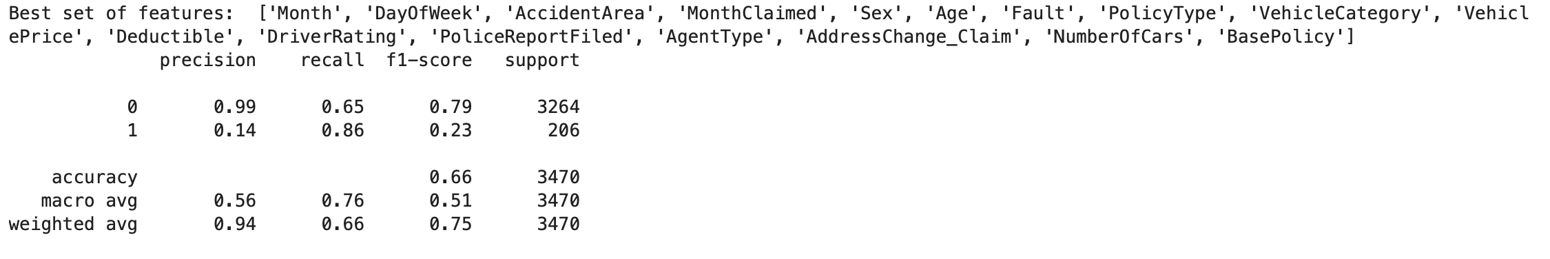
Interpretation: Class 0 (Non-Fraudulent Claims): The model performs well in identifying non-fraudulent claims with high precision (0.99) and moderate recall (0.65), resulting in a relatively high F1-score (0.79). This suggests that it correctly identifies most non-fraudulent claims but misses some.

Class 1 (Fraudulent Claims): The model’s performance is poor for fraudulent claims, with low precision (0.14) and a high recall (0.86), resulting in a low F1-score (0.23). This indicates that it incorrectly identifies many non-fraudulent claims as fraudulent.

Implication: High false positive rates (predicting non-fraudulent claims as fraudulent) can lead to unnecessary investigations and strain on resources. Moreover, the model’s inability to capture a substantial portion of fraudulent claims (low recall) suggests potential financial risks due to undetected fraudulent activities.

Random forest

import pandas as pd
import numpy as np
import matplotlib.pyplot as plt
import seaborn as sns
from sklearn.pipeline import Pipeline
from sklearn.compose import ColumnTransformer
from sklearn.impute import SimpleImputer
from sklearn.preprocessing import StandardScaler
from sklearn.metrics import classification_report, confusion_matrix, roc_curve, auc
from sklearn.model_selection import train_test_split, cross_val_predict, GridSearchCV
from sklearn.ensemble import RandomForestClassifier
from sklearn.utils.class_weight import compute_class_weight



# Assign unique integer values to all non-numeric values in the DataFrame
for col in df_processed.select_dtypes(include=['object']).columns:
    unique_values = df_processed[col].unique()
    value_map = {value: i for i, value in enumerate(unique_values)}
    df_processed[col] = df_processed[col].map(value_map)

# Define features and target
X = df_processed.drop('FraudFound_P', axis=1)
y = df_processed['FraudFound_P']

# Split the data into training and testing sets with stratify
X_train, X_test, y_train, y_test = train_test_split(X, y, test_size=0.3, random_state=42, stratify=y)

# Compute class weights based on the training set
class_weights = compute_class_weight(class_weight='balanced', classes=np.unique(y_train), y=y_train)
class_weights_dict = {i: class_weights[i] for i in range(len(class_weights))}

# Function to perform stepwise feature selection and evaluation for Random Forest
def evaluate_random_forest_with_stepwise_selection(param_grid):
    # Initialize variables for the stepwise feature selection
    best_features = []
    best_score = 0
    threshold_score = 0.6

    # Iterate over all features
    for feature in X.columns:
        # Add the new feature to the list of best features
        features_to_try = best_features + [feature]
        
        # Create a pipeline with the current set of features
        current_pipeline = Pipeline(steps=[
            ('preprocessor', ColumnTransformer(
                transformers=[
                    ('num', Pipeline(steps=[
                        ('imputer', SimpleImputer(strategy='median')),
                        ('scaler', StandardScaler())
                    ]), X[features_to_try].select_dtypes(include=['float64', 'int64']).columns),
                    ('cat', Pipeline(steps=[
                        ('imputer', SimpleImputer(strategy='constant', fill_value=0))
                    ]), X[features_to_try].select_dtypes(include=['int']).columns)
                ]
            )),
            ('classifier', RandomForestClassifier(random_state=42, n_jobs=-1, class_weight=class_weights_dict))
        ])
        
        # Setup Grid Search with cross-validation
        grid_search = GridSearchCV(current_pipeline, param_grid, cv=5, scoring='roc_auc', n_jobs=-1, verbose=0)
        
        # Fit the model
        grid_search.fit(X_train[features_to_try], y_train)
        
        # Get the best score
        score = grid_search.best_score_
        
        # If the performance improves and is above the threshold, keep the feature
        if score > best_score and score >= threshold_score:
            best_score = score
            best_features.append(feature)
            print(f"Random Forest - Added feature: {feature} - New best score: {best_score}")

    # Print the final set of best features
    print("Random Forest - Best set of features: ", best_features)

    # Create a final pipeline with the best features
    final_pipeline = Pipeline(steps=[
        ('preprocessor', ColumnTransformer(
            transformers=[
                ('num', Pipeline(steps=[
                    ('imputer', SimpleImputer(strategy='median')),
                    ('scaler', StandardScaler())
                ]), X[best_features].select_dtypes(include=['float64', 'int64']).columns),
                ('cat', Pipeline(steps=[
                    ('imputer', SimpleImputer(strategy='constant', fill_value=0))
                ]), X[best_features].select_dtypes(include=['int']).columns)
            ]
        )),
        ('classifier', RandomForestClassifier(random_state=42, n_jobs=-1, class_weight=class_weights_dict))
    ])

    # Fit the final pipeline with the best features
    final_pipeline.fit(X_train[best_features], y_train)

    # Predict and evaluate using the final model
    y_pred = final_pipeline.predict(X_test[best_features])
    print(classification_report(y_test, y_pred))

    # Generate cross-validated predictions for ROC AUC curve using the best model
    y_scores = cross_val_predict(final_pipeline, X_train[best_features], y_train, cv=5, method='predict_proba')[:, 1]

    # Compute ROC curve and ROC AUC
    fpr, tpr, thresholds = roc_curve(y_train, y_scores)
    roc_auc = auc(fpr, tpr)

    # Plot ROC AUC curve
    plt.figure()
    plt.plot(fpr, tpr, color='darkorange', lw=2, label='ROC curve (area = %0.2f)' % roc_auc)
    plt.plot([0, 1], [0, 1], color='navy', lw=2, linestyle='--')
    plt.xlim([0.0, 1.0])
    plt.ylim([0.0, 1.05])
    plt.xlabel('False Positive Rate')
    plt.ylabel('True Positive Rate')
    plt.title('Receiver Operating Characteristic (ROC) Curve - Random Forest')
    plt.legend(loc="lower right")
    plt.show()

    # Confusion matrix with labels and percentages
    cm = confusion_matrix(y_test, y_pred)
    class_names = ['Legit', 'Fraud']

    # Plot confusion matrix with counts and percentages
    plt.figure(figsize=(8, 6))
    sns.heatmap(cm, annot=True, fmt='d', cmap='Blues', xticklabels=class_names, yticklabels=class_names)
    plt.xlabel('Predicted labels')
    plt.ylabel('True labels')
    plt.title('Confusion Matrix (Class Counts and Percentages) - Random Forest')

    # Calculate class percentages
    class_percentages = cm / cm.sum(axis=1)[:, np.newaxis]

    # Add text annotations for class percentages
    for i in range(cm.shape[0]):
        for j in range(cm.shape[1]):
            if cm[i, j] != 0:
                percentage = class_percentages[i, j]
                plt.text(j + 0.5, i + 0.2, f'{percentage:.2%}', 
                         horizontalalignment='center', verticalalignment='center', color='green')

    plt.show()

# Random Forest parameters for Grid Search
rf_param_grid = {
    "classifier__n_estimators": [100, 200],
    "classifier__max_depth": [None, 10, 20],
    "classifier__min_samples_split": [2, 5, 10]
}

# Evaluate Random Forest with stepwise feature selection
evaluate_random_forest_with_stepwise_selection(rf_param_grid)

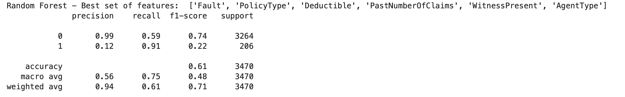
The set of best features used and their result: data info Interpretation Class 0 (Non-Fraudulent Claims): The model performs exceptionally well in identifying non-fraudulent claims with very high precision (0.99), but it has moderate recall (0.59). This means while most of the predicted non-fraudulent claims are indeed non-fraudulent, it misses a significant portion of actual non-fraudulent claims.

Class 1 (Fraudulent Claims): The model has a low precision (0.12) for fraudulent claims, indicating a high number of false positives. However, it has a very high recall (0.91), meaning it successfully identifies most actual fraudulent claims. The F1-score (0.22) suggests a poor balance between precision and recall for fraudulent claims Balance Interpretation: The high recall (0.91) suggests that the model is effective in capturing a large portion of fraudulent activity. However, the low precision (0.12) indicates a high rate of false positives, where legitimate claims are misclassified as fraudulent.

Implications: While the high recall is beneficial for identifying actual fraudulent claims, the low precision can lead to unnecessary investigations or denials for legitimate claims. Achieving a better balance between recall and precision for class 1 is essential to reduce false positives while maintaining a high capture rate of fraudulent activities.

Xgboost

import pandas as pd
import numpy as np
import matplotlib.pyplot as plt
import seaborn as sns
from sklearn.pipeline import Pipeline
from sklearn.compose import ColumnTransformer
from sklearn.impute import SimpleImputer
from sklearn.preprocessing import StandardScaler
from sklearn.metrics import classification_report, roc_curve, auc
from sklearn.model_selection import train_test_split, cross_val_predict, GridSearchCV
from xgboost import XGBClassifier
from imblearn.over_sampling import SMOTE



# Assign unique integer values to all non-numeric values in the DataFrame
for col in df_processed.select_dtypes(include=['object']).columns:
    unique_values = df_processed[col].unique()
    value_map = {value: i for i, value in enumerate(unique_values)}
    df_processed[col] = df_processed[col].map(value_map)

# Define features and target
X = df_processed.drop('FraudFound_P', axis=1)
y = df_processed['FraudFound_P']

# Split the data into training and testing sets with stratify
X_train, X_test, y_train, y_test = train_test_split(X, y, test_size=0.3, random_state=42, stratify=y)


# Calculate the scale_pos_weight dynamically
neg_count = (y_train == 0).sum()
pos_count = (y_train == 1).sum()
scale_pos_weight = neg_count / pos_count
print(f"Calculated scale_pos_weight: {scale_pos_weight}")

# Initialize variables for the stepwise feature selection
best_features = []
best_score = 0
threshold_score = 0.6

# Define the XGBoost parameters for Grid Search
param_grid = {
    "classifier__n_estimators": [100, 200],
    "classifier__learning_rate": [0.01, 0.1],
    "classifier__max_depth": [3, 5]
    
}

# Iterate over all features
for feature in X.columns:
    # Add the new feature to the list of best features
    features_to_try = best_features + [feature]
    
    # Create a pipeline with the current set of features
    current_pipeline = Pipeline(steps=[
        ('preprocessor', ColumnTransformer(
            transformers=[
                ('num', Pipeline(steps=[
                    ('imputer', SimpleImputer(strategy='median')),
                    ('scaler', StandardScaler())
                ]), X[features_to_try].select_dtypes(include=['float64', 'int64']).columns),
                ('cat', Pipeline(steps=[
                    ('imputer', SimpleImputer(strategy='constant', fill_value=0))
                ]), X[features_to_try].select_dtypes(include=['int']).columns)
            ]
        )),
        ('classifier', XGBClassifier(random_state=42, objective='binary:logistic', n_jobs=-1))
    ])
    
    # Setup Grid Search with cross-validation
    grid_search = GridSearchCV(current_pipeline, param_grid, cv=5, scoring='roc_auc', n_jobs=-1, verbose=0)
    
    # Fit the model
    grid_search.fit(X_train[features_to_try], y_train)
    
    # Get the best score
    score = grid_search.best_score_
    
    # If the performance improves and is above the threshold, keep the feature
    if score > best_score and score >= threshold_score:
        best_score = score
        best_features.append(feature)
        print(f"Added feature: {feature} - New best score: {best_score}")

# Print the final set of best features
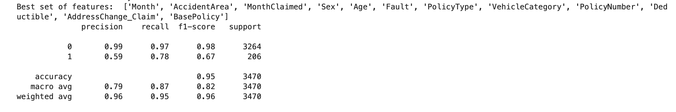
print("Best set of features: ", best_features)

# Create a final pipeline with the best features
final_pipeline = Pipeline(steps=[
    ('preprocessor', ColumnTransformer(
        transformers=[
            ('num', Pipeline(steps=[
                ('imputer', SimpleImputer(strategy='median')),
                ('scaler', StandardScaler())
            ]), X[best_features].select_dtypes(include=['float64', 'int64']).columns),
            ('cat', Pipeline(steps=[
                ('imputer', SimpleImputer(strategy='constant', fill_value=0))
            ]), X[best_features].select_dtypes(include=['int']).columns)
        ]
    )),
    ('classifier', XGBClassifier(random_state=42, objective='binary:logistic', n_jobs=-1,scale_pos_weight=scale_pos_weight,))
])

# Fit the final pipeline with the best features
final_pipeline.fit(X_train[best_features], y_train)

# Predict and evaluate using the final model
y_pred = final_pipeline.predict(X_test[best_features])
print(classification_report(y_test, y_pred))

# Generate cross-validated predictions for ROC AUC curve using the best model
y_scores = cross_val_predict(final_pipeline, X_train[best_features], y_train, cv=5, method='predict_proba')[:, 1]
# save the trained pipeline
joblib.dump(final_pipeline, 'xgboost_model_pipeline.pkl')

# Compute ROC curve and ROC AUC
fpr, tpr, thresholds = roc_curve(y_train, y_scores)
roc_auc = auc(fpr, tpr)

# Plot ROC AUC curve
plt.figure()
plt.plot(fpr, tpr, color='darkorange', lw=2, label='ROC curve (area = %0.2f)' % roc_auc)
plt.plot([0, 1], [0, 1], color='navy', lw=2, linestyle='--')
plt.xlim([0.0, 1.0])
plt.ylim([0.0, 1.05])
plt.xlabel('False Positive Rate')
plt.ylabel('True Positive Rate')
plt.title('Receiver Operating Characteristic (ROC) Curve')
plt.legend(loc="lower right")
plt.show()

The set of best features used and their result: data info ** Interpretation Class 0 (Non-Fraudulent Claims): The model performs exceptionally well in identifying non-fraudulent claims, with very high precision (0.99) and recall (0.97). This results in a high F1-score (0.98), indicating a strong balance between precision and recall for non-fraudulent claims.

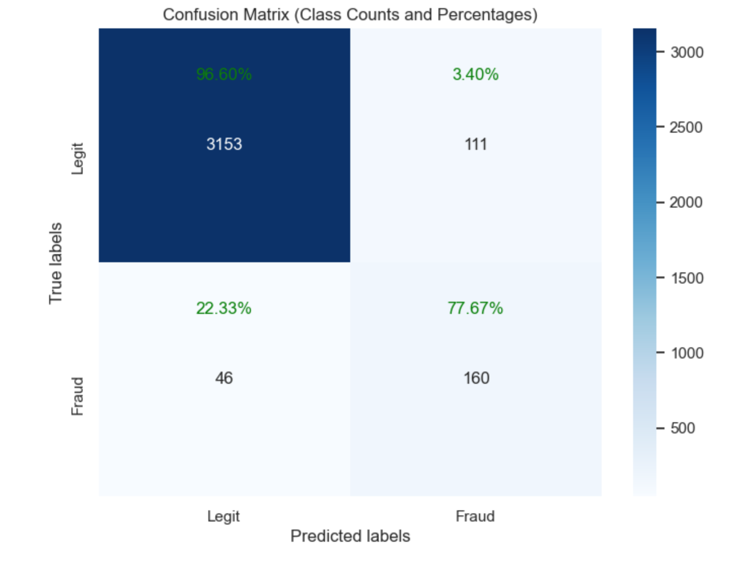
Class 1 (Fraudulent Claims): The model has a moderate precision (0.59) for fraudulent claims, meaning that there are still some false positives. However, the recall (0.78) is relatively high, indicating that the model successfully identifies a significant portion of actual fraudulent claims. The F1-score (0.67) suggests a reasonable balance between precision and recall for fraudulent claims, though there is room for improvement, especially in reducing false positives.

Overall Metrics: The accuracy (0.95) is very high, reflecting the model’s strong overall performance. The macro average metrics provide a balanced view of the model’s performance across both classes, indicating an overall good performance but highlighting that the model is slightly better at predicting non-fraudulent claims. The weighted average metrics, accounting for class imbalance, are also very high, showing that the model performs well overall.

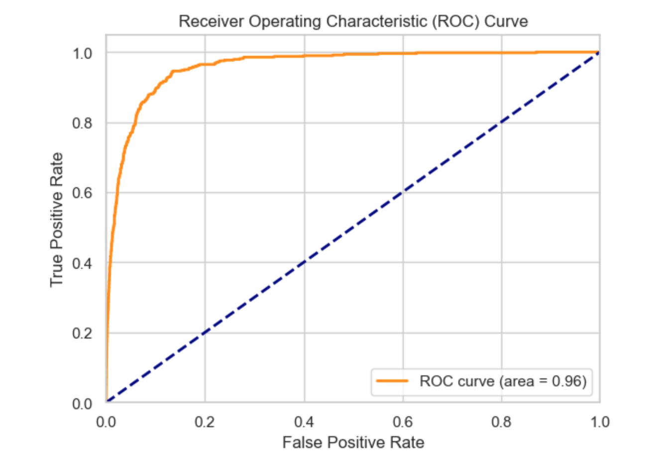
data info An AUC (Area Under the ROC Curve) of 0.96 indicates that the model is highly effective at distinguishing between positive and negative classes. Practically, this means that if you randomly select one positive instance (such as a fraudulent claim) and one negative instance (such as a legitimate claim), the model has a 96% chance of correctly ranking the positive instance higher than the negative one. This level of performance suggests that the model is very reliable and can be trusted for practical applications in predicting fraudulent insurance claims.

Selecting the best algorithm

When selecting an algorithm for the inference pipeline, it’s crucial to strike a balance between recall and precision, depending on the specific goals and constraints of the application. In practice, any of the following could arise;

High precision - low recall: High precision means that the model is very accurate when it predicts a positive case (e.g., a fraudulent claim). However, low recall indicates that the model misses many actual positive cases. This scenario implies that the model is conservative in making positive predictions, which has both advantages and disadvantages.

High precision and high recall: High precision and high recall together signify that the model is highly effective in predicting positive cases (e.g., fraudulent claims) and is also excellent at identifying almost all actual positive cases. Achieving both high precision and high recall is the ideal scenario in classification problems, though it is often challenging.

Low precision - high recall: Low precision means that many of the cases predicted as positive (fraudulent claims) are actually negative (legitimate claims). High recall indicates that the model successfully identifies most of the actual positive cases. This scenario suggests the model is aggressive in flagging potential fraud. (Hint: Refer to the scores from the random forest and logistics models in this tutorial).

Low Precision - Low Recall: Low precision and low recall together indicate that the model performs poorly in predicting positive cases (e.g., fraudulent claims) and fails to identify most of the actual positive cases. This is the least desirable scenario for any classification problem.

A balanced precision-recall score: Achieving a balance between precision and recall means that the model effectively identifies a substantial portion of fraudulent claims while maintaining a reasonable number of false positives. This balance is often sought in practice to ensure both comprehensive detection and operational efficiency. (Hint: Refer to the scores from the xgboost model)

Conclusion

In conclusion, the XGBoost algorithm has proven to be highly effective at identifying potential fraudulent claims, as evidenced by the following:

Superior Performance: The model achieves high precision, recall, and F1-scores for both non-fraudulent and fraudulent claims, indicating balanced performance. The high overall accuracy and weighted averages demonstrate the model’s robustness and reliability.

Enhanced Fraud Detection: The significant improvement in recall for fraudulent claims means that the model effectively captures more fraudulent activities, thereby reducing financial risks associated with undetected fraud.

High AUC: The AUC of 0.96 confirms the model’s outstanding ability to distinguish between fraudulent and non-fraudulent claims, making it highly suitable for real-world applications.

Operational Efficiency(balanced precision-recall tradeoff): High precision for non-fraudulent claims ensures efficient processing of legitimate claims, minimizing unnecessary investigations and operational costs.

In the next tutorial, we will develop a web-based application based on the XGBoost model. This application will enable users to determine whether a claim is legitimate or possibly fraudulent by either uploading an Excel sheet or entering a policy number. See you in the next one!